第5章重回帰モデルの推定と検定

先に出版社サイトよりデータをダウンロードする.

# サポートファイルへのリンク
curl <- "https://www.yuhikaku.co.jp/static_files/05385_support05.zip"
# ダウンロード保存用フォルダが存在しない場合, 作成
if(!dir.exists("downloads")){
    dir.create("downloads")
}
cdestfile <- "downloads/support05.zip"
download.file(curl, cdestfile)
# データ保存用フォルダが存在しない場合, 作成
if(!dir.exists("data")){
    dir.create("data")
}
# WSL上のRで解凍すると文字化けするので、Linuxのコマンドを外部呼び出し
# Windowsの場合は別途コマンドを用いる.
if(.Platform$OS.type == "unix") {
    system(sprintf('unzip -n -Ocp932 %s -d %s', "downloads/support05.zip", "./data"))
} else {
    print("Windowsで解凍するコマンドを別途追加せよ.")
}

必要なライブラリを読み込む.

library(tidyverse)
library(estimatr)
library(knitr)
library(modelsummary)
## `modelsummary` 2.0.0 now uses `tinytable` as its default table-drawing
##   backend. Learn more at: https://vincentarelbundock.github.io/tinytable/
## 
## Revert to `kableExtra` for one session:
## 
##   options(modelsummary_factory_default = 'kableExtra')
##   options(modelsummary_factory_latex = 'kableExtra')
##   options(modelsummary_factory_html = 'kableExtra')
## 
## Silence this message forever:
## 
##   config_modelsummary(startup_message = FALSE)
library(gt)
library(car)
## Loading required package: carData
## 
## Attaching package: 'car'
## The following object is masked from 'package:dplyr':
## 
##     recode
## The following object is masked from 'package:purrr':
## 
##     some
library(wooldridge)
library(haven)
library(kableExtra)
## 
## Attaching package: 'kableExtra'
## The following object is masked from 'package:dplyr':
## 
##     group_rows

単回帰 (5.1), (5.2)

先にデータを読み込み, 変数を作成する.

youdou <- read.csv("data/05_第5章/youdou.csv")
youdou <- youdou %>%
    mutate(lny80 = log(y80)) %>%
    mutate(lny99 = log(y99)) %>%
    mutate(lny90 = log(y90)) %>%
    mutate(growthrate8099 = (lny99-lny80)/19*100) %>%
    mutate(growthrate8090 = (lny90-lny80)/10)

不均一分散に頑健な標準誤差を求めるために, estimatr::lm_robust()を使う.

youdou_51 <- lm_robust(growthrate8099 ~ trust80, data = youdou, se_type = "stata")
summary(youdou_51)
## 
## Call:
## lm_robust(formula = growthrate8099 ~ trust80, data = youdou, 
##     se_type = "stata")
## 
## Standard error type:  HC1 
## 
## Coefficients:
##             Estimate Std. Error t value  Pr(>|t|) CI Lower CI Upper DF
## (Intercept)   3.1394    0.06044  51.943 8.188e-42  3.01763   3.2611 45
## trust80       0.2247    0.06640   3.384 1.491e-03  0.09094   0.3584 45
## 
## Multiple R-squared:  0.179 , Adjusted R-squared:  0.1608 
## F-statistic: 11.45 on 1 and 45 DF,  p-value: 0.001491
youdou_52 <- lm_robust(growthrate8099 ~ norm80, data = youdou, se_type = "stata")
summary(youdou_52)
## 
## Call:
## lm_robust(formula = growthrate8099 ~ norm80, data = youdou, se_type = "stata")
## 
## Standard error type:  HC1 
## 
## Coefficients:
##             Estimate Std. Error t value  Pr(>|t|) CI Lower CI Upper DF
## (Intercept)   3.0905    0.04826  64.033 7.544e-46   2.9933   3.1878 45
## norm80        0.5597    0.07058   7.931 4.348e-10   0.4176   0.7019 45
## 
## Multiple R-squared:  0.4563 ,    Adjusted R-squared:  0.4442 
## F-statistic:  62.9 on 1 and 45 DF,  p-value: 4.348e-10

実証例5.1 信頼と規範が経済成長に与える影響の重回帰分析

youdou_55 <- lm_robust(growthrate8099 ~ trust80 + education80 + lny80, data = youdou, se_type = "stata")
summary(youdou_55)
## 
## Call:
## lm_robust(formula = growthrate8099 ~ trust80 + education80 + 
##     lny80, data = youdou, se_type = "stata")
## 
## Standard error type:  HC1 
## 
## Coefficients:
##             Estimate Std. Error t value  Pr(>|t|) CI Lower CI Upper DF
## (Intercept)  6.04885    0.42643 14.1849 8.041e-18    5.189   6.9088 43
## trust80      0.02058    0.07564  0.2721 7.868e-01   -0.132   0.1731 43
## education80  2.61208    2.70857  0.9644 3.403e-01   -2.850   8.0744 43
## lny80       -2.38309    0.49147 -4.8489 1.658e-05   -3.374  -1.3920 43
## 
## Multiple R-squared:  0.5619 ,    Adjusted R-squared:  0.5313 
## F-statistic: 20.21 on 3 and 43 DF,  p-value: 2.531e-08
youdou_55_2 <- lm_robust(growthrate8099 ~ norm80 + education80 + lny80, data = youdou, se_type = "stata")
summary(youdou_55_2)
## 
## Call:
## lm_robust(formula = growthrate8099 ~ norm80 + education80 + lny80, 
##     data = youdou, se_type = "stata")
## 
## Standard error type:  HC1 
## 
## Coefficients:
##             Estimate Std. Error t value  Pr(>|t|) CI Lower CI Upper DF
## (Intercept)   5.2909     0.6682   7.918 6.204e-10  3.94324   6.6385 43
## norm80        0.3383     0.1370   2.469 1.758e-02  0.06202   0.6145 43
## education80   4.3872     1.9611   2.237 3.051e-02  0.43233   8.3421 43
## lny80        -1.9911     0.5746  -3.465 1.213e-03 -3.14987  -0.8324 43
## 
## Multiple R-squared:  0.6391 ,    Adjusted R-squared:  0.614 
## F-statistic: 41.04 on 3 and 43 DF,  p-value: 1.11e-12

実証例5.2 FWL定理の確認

定数項なしの回帰を実行するには, formulaに+0か-1を追加する(参考). なお, estimatr::lm_robust()にはlmのようにresidualsがないため, 必要ならば手動で追加する(参考). ただしこの例では標準偏差は必要でないため, lmを用いた.

fwl_1 <- lm(trust80 ~ education80 + lny80, data = youdou)
summary(fwl_1)
## 
## Call:
## lm(formula = trust80 ~ education80 + lny80, data = youdou)
## 
## Residuals:
##      Min       1Q   Median       3Q      Max 
## -1.18774 -0.48567 -0.02193  0.56490  1.41091 
## 
## Coefficients:
##             Estimate Std. Error t value Pr(>|t|)   
## (Intercept)   2.6740     0.9493   2.817  0.00723 **
## education80 -11.2886     4.5080  -2.504  0.01606 * 
## lny80        -1.0254     0.9692  -1.058  0.29584   
## ---
## Signif. codes:  0 '***' 0.001 '**' 0.01 '*' 0.05 '.' 0.1 ' ' 1
## 
## Residual standard error: 0.6555 on 44 degrees of freedom
## Multiple R-squared:  0.4246, Adjusted R-squared:  0.3985 
## F-statistic: 16.24 on 2 and 44 DF,  p-value: 5.233e-06
fwl_2 <- lm(growthrate8099 ~ education80 + lny80, data = youdou)
summary(fwl_2)
## 
## Call:
## lm(formula = growthrate8099 ~ education80 + lny80, data = youdou)
## 
## Residuals:
##      Min       1Q   Median       3Q      Max 
## -0.46861 -0.23426  0.00308  0.13266  1.01937 
## 
## Coefficients:
##             Estimate Std. Error t value Pr(>|t|)    
## (Intercept)   6.1039     0.4403  13.863  < 2e-16 ***
## education80   2.3797     2.0909   1.138    0.261    
## lny80        -2.4042     0.4495  -5.348 3.03e-06 ***
## ---
## Signif. codes:  0 '***' 0.001 '**' 0.01 '*' 0.05 '.' 0.1 ' ' 1
## 
## Residual standard error: 0.304 on 44 degrees of freedom
## Multiple R-squared:  0.561,  Adjusted R-squared:  0.5411 
## F-statistic: 28.12 on 2 and 44 DF,  p-value: 1.36e-08
lm(fwl_2$residuals ~ 0 + fwl_1$residuals) %>% summary()
## 
## Call:
## lm(formula = fwl_2$residuals ~ 0 + fwl_1$residuals)
## 
## Residuals:
##      Min       1Q   Median       3Q      Max 
## -0.45839 -0.21925 -0.00947  0.13042  1.03231 
## 
## Coefficients:
##                 Estimate Std. Error t value Pr(>|t|)
## fwl_1$residuals  0.02058    0.06832   0.301    0.765
## 
## Residual standard error: 0.2971 on 46 degrees of freedom
## Multiple R-squared:  0.00197,    Adjusted R-squared:  -0.01973 
## F-statistic: 0.09078 on 1 and 46 DF,  p-value: 0.7645

実証例5.3 FWL定理の別表現の確認

lm(growthrate8099 ~ fwl_1$residuals-1, data = youdou) %>% summary()
## 
## Call:
## lm(formula = growthrate8099 ~ fwl_1$residuals - 1, data = youdou)
## 
## Residuals:
##    Min     1Q Median     3Q    Max 
##  2.189  2.816  3.086  3.546  3.915 
## 
## Coefficients:
##                 Estimate Std. Error t value Pr(>|t|)
## fwl_1$residuals  0.02058    0.73877   0.028    0.978
## 
## Residual standard error: 3.212 on 46 degrees of freedom
## Multiple R-squared:  1.688e-05,  Adjusted R-squared:  -0.02172 
## F-statistic: 0.0007764 on 1 and 46 DF,  p-value: 0.9779

実証例5.4 信頼と規範が経済成長に与える影響の重回帰分析の標準誤差

実証例5.1を参照せよ.

実証例5.5 信頼と規範が経済成長に与える影響の多項式モデル

youdou_515 <- lm_robust(growthrate8099 ~ y80 + I(y80^2), data = youdou, se_type = "stata")
summary(youdou_515)
## 
## Call:
## lm_robust(formula = growthrate8099 ~ y80 + I(y80^2), data = youdou, 
##     se_type = "stata")
## 
## Standard error type:  HC1 
## 
## Coefficients:
##             Estimate Std. Error t value  Pr(>|t|) CI Lower CI Upper DF
## (Intercept)  6.51866    1.38538   4.705 2.535e-05  3.72662   9.3107 44
## y80         -1.22615    0.70791  -1.732 9.027e-02 -2.65285   0.2005 44
## I(y80^2)     0.08935    0.08861   1.008 3.188e-01 -0.08923   0.2679 44
## 
## Multiple R-squared:  0.5503 ,    Adjusted R-squared:  0.5299 
## F-statistic: 27.39 on 2 and 44 DF,  p-value: 1.879e-08

図5-1 散布図と推定された回帰曲線

youdou %>%
    ggplot(aes(x = y80, y = growthrate8099)) +
    geom_point() +
    xlab("初期時点GDP") +
    ylab("経済成長率") +
    geom_smooth(method = "lm", formula = y ~ x + I(x^2), se = FALSE, color = "black")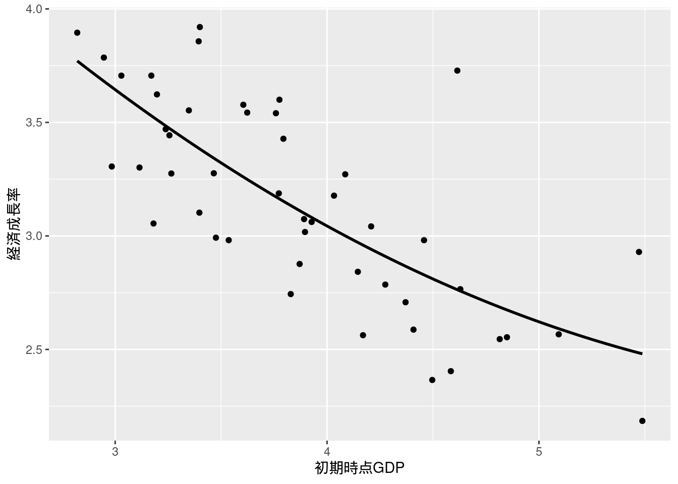

例題5.5

lm_robust(growthrate8099 ~ lny80 * education80, data = youdou, se_type = "stata") %>% summary()
## 
## Call:
## lm_robust(formula = growthrate8099 ~ lny80 * education80, data = youdou, 
##     se_type = "stata")
## 
## Standard error type:  HC1 
## 
## Coefficients:
##                   Estimate Std. Error  t value  Pr(>|t|) CI Lower CI Upper DF
## (Intercept)         6.0868     1.1220  5.42485 2.492e-06    3.824   8.3496 43
## lny80              -2.3937     0.8477 -2.82364 7.167e-03   -4.103  -0.6841 43
## education80         2.5735    11.0413  0.23308 8.168e-01  -19.693  24.8405 43
## lny80:education80  -0.1211     7.1314 -0.01698 9.865e-01  -14.503  14.2608 43
## 
## Multiple R-squared:  0.561 , Adjusted R-squared:  0.5304 
## F-statistic: 18.45 on 3 and 43 DF,  p-value: 7.651e-08

実証例5.6 都市化の度合いと初期時点GDPの交互作用

先にダミー変数urbanを作成してから回帰分析を実行する(下ではurbanの型はintではなくboolになるが構わない). urbanの値により標本を分ける場合は, lm()のdataでfilter()を使えばよい.

youdou <- youdou %>%
    mutate(urban = did > 0.4)
lm(growthrate8099 ~ urban * lny80, data = youdou) %>% summary()
## 
## Call:
## lm(formula = growthrate8099 ~ urban * lny80, data = youdou)
## 
## Residuals:
##      Min       1Q   Median       3Q      Max 
## -0.51040 -0.21003 -0.02406  0.16516  0.90189 
## 
## Coefficients:
##                 Estimate Std. Error t value Pr(>|t|)    
## (Intercept)      5.74905    0.57763   9.953 9.96e-13 ***
## urbanTRUE       -0.17551    0.82444  -0.213 0.832421    
## lny80           -1.91120    0.45104  -4.237 0.000117 ***
## urbanTRUE:lny80  0.06441    0.61108   0.105 0.916546    
## ---
## Signif. codes:  0 '***' 0.001 '**' 0.01 '*' 0.05 '.' 0.1 ' ' 1
## 
## Residual standard error: 0.3092 on 43 degrees of freedom
## Multiple R-squared:  0.5564, Adjusted R-squared:  0.5254 
## F-statistic: 17.98 on 3 and 43 DF,  p-value: 1.041e-07
lm(growthrate8099 ~ lny80, data = (youdou %>% filter(!urban))) %>% summary()
## 
## Call:
## lm(formula = growthrate8099 ~ lny80, data = (youdou %>% filter(!urban)))
## 
## Residuals:
##      Min       1Q   Median       3Q      Max 
## -0.51040 -0.22240 -0.02406  0.12827  0.90189 
## 
## Coefficients:
##             Estimate Std. Error t value Pr(>|t|)    
## (Intercept)   5.7491     0.6512   8.829 7.59e-09 ***
## lny80        -1.9112     0.5085  -3.759  0.00102 ** 
## ---
## Signif. codes:  0 '***' 0.001 '**' 0.01 '*' 0.05 '.' 0.1 ' ' 1
## 
## Residual standard error: 0.3486 on 23 degrees of freedom
## Multiple R-squared:  0.3805, Adjusted R-squared:  0.3536 
## F-statistic: 14.13 on 1 and 23 DF,  p-value: 0.001022
lm(growthrate8099 ~ lny80, data = (youdou %>% filter(urban))) %>% summary()
## 
## Call:
## lm(formula = growthrate8099 ~ lny80, data = (youdou %>% filter(urban)))
## 
## Residuals:
##      Min       1Q   Median       3Q      Max 
## -0.35740 -0.19171 -0.05236  0.17634  0.49475 
## 
## Coefficients:
##             Estimate Std. Error t value Pr(>|t|)    
## (Intercept)   5.5735     0.4881  11.419 3.25e-10 ***
## lny80        -1.8468     0.3421  -5.399 2.77e-05 ***
## ---
## Signif. codes:  0 '***' 0.001 '**' 0.01 '*' 0.05 '.' 0.1 ' ' 1
## 
## Residual standard error: 0.2565 on 20 degrees of freedom
## Multiple R-squared:  0.593,  Adjusted R-squared:  0.5727 
## F-statistic: 29.14 on 1 and 20 DF,  p-value: 2.769e-05

実証例5.7 都市化の度合いと初期時点GDPのダミー変数同士の交互作用

やはり, 先にダミー変数lny80dを作成する.

youdou <- youdou %>%
    mutate(lny80d = lny80 > 1.4)
lm(growthrate8099 ~ urban * lny80d, data = youdou) %>% summary()
## 
## Call:
## lm(formula = growthrate8099 ~ urban * lny80d, data = youdou)
## 
## Residuals:
##      Min       1Q   Median       3Q      Max 
## -0.50919 -0.25376 -0.01148  0.24475  0.85353 
## 
## Coefficients:
##                      Estimate Std. Error t value Pr(>|t|)    
## (Intercept)           3.45474    0.07544  45.793  < 2e-16 ***
## urbanTRUE            -0.23329    0.12459  -1.872 0.067953 .  
## lny80dTRUE           -0.58003    0.15400  -3.767 0.000498 ***
## urbanTRUE:lny80dTRUE  0.04725    0.20827   0.227 0.821596    
## ---
## Signif. codes:  0 '***' 0.001 '**' 0.01 '*' 0.05 '.' 0.1 ' ' 1
## 
## Residual standard error: 0.3288 on 43 degrees of freedom
## Multiple R-squared:  0.4982, Adjusted R-squared:  0.4631 
## F-statistic: 14.23 on 3 and 43 DF,  p-value: 1.401e-06

実証例5.8 非線形モデルにおける結合仮説の検定

実証例5.5を参照せよ.

実証例5.9 ポンフェローニ検定

式は実証例5.1を参照せよ. 規範と教育水準の係数が両方とも0であるという帰無仮説を検定する. F検定統計値はcar::linearHypothesis()を使うことで求められる.

linearHypothesis(youdou_55_2, c("norm80","education80"), test = "F")
## 
## Linear hypothesis test:
## norm80 = 0
## education80 = 0
## 
## Model 1: restricted model
## Model 2: growthrate8099 ~ norm80 + education80 + lny80
## 
##   Res.Df Df      F   Pr(>F)   
## 1     45                      
## 2     43  2 5.4375 0.007848 **
## ---
## Signif. codes:  0 '***' 0.001 '**' 0.01 '*' 0.05 '.' 0.1 ' ' 1

表5-5 記述統計量

modelsummary::datasummary()を使うことで簡単に記述統計表が作成できる. ここでは統計量と変数名の表示を日本語に直すため, 一旦dataframeで書き出し, 再度gtで修正した表を表示している.

# 変数を選択
vars <- youdou %>%
    select(growthrate8099, trust80, norm80, education80, lny80)
table55 <- datasummary(All(vars) ~ N + Mean + SD + Min + Max,
            data = youdou,
            output = "data.frame",
            fmt = 3)
# 列名
colnames(table55) <- c("変数", "サンプルサイズ", "平均", "標準偏差", "最小値", "最大値")
# 変数名
table55[,1] <- c("経済成長率", "信頼", "規範", "教育水準", "初期時点対数GDP")
# 表を出力
gt(table55)

変数	サンプルサイズ	平均	標準偏差	最小値	最大値
経済成長率	47	3.147	0.449	2.185	3.920
信頼	47	0.033	0.845	-1.668	1.918
規範	47	0.101	0.542	-1.248	1.297
教育水準	47	0.112	0.036	0.069	0.238
初期時点対数GDP	47	1.341	0.167	1.037	1.703

表5-6 推定結果: 被説明変数は経済成長率

回帰結果の表はmodelsummaryを使う (stargazerでも可能だが更新が止まっており, estimatrの結果を表示できないなどデメリットがある). modelsummary::msummary()のgoef_omitで表示しない統計量を指定できるが, これは正規表現を使っているため, 自由度修正済み決定係数$\bar{R}^2$を表示し, 通常の決定係数$R^2$を表示させないためにはR2$とすればよい. F検定統計量の値を表示するにあたっては, このサイトを参考にした.

models <- list(
    "(1)" = lm_robust(growthrate8099 ~ trust80, data = youdou, se_type = "stata"),
    "(2)" = lm_robust(growthrate8099 ~ norm80, data = youdou, se_type = "stata"),
    "(3)" = lm_robust(growthrate8099 ~ trust80 + norm80, data = youdou, se_type = "stata"),
    "(4)" = lm_robust(growthrate8099 ~ trust80 + lny80 + education80, data = youdou, se_type = "stata"),
    "(5)" = lm_robust(growthrate8099 ~ norm80 + lny80 + education80, data = youdou, se_type = "stata"),
    "(6)" = lm_robust(growthrate8099 ~ trust80 + norm80 + lny80 + education80, data = youdou, se_type = "stata"))

# F検定統計量の値を表示するモデルを指定
attr(models[3]$`(3)`, "FTEST") <- TRUE
attr(models[6]$`(6)`, "FTEST") <- TRUE

glance_custom.lm_robust <- function(x) {
    # 上で指定した, F検定統計量の値を表示したいモデルでなければパス
    if (!isTRUE(attr(x, "FTEST"))) return(NULL)

    # F検定を実行
    ftest <- linearHypothesis(x, test = "F", c("trust80", "norm80"))

    # F検定統計量の値とp値をまとめたtibbleを作成
    out <- tibble(
        "F検定統計量の値 $H_0: \\beta_{信頼}=0, \\beta_{規範}=0$" = ftest[["F"]][2],
        "     " = sprintf("(%.3f)", ftest[["Pr(>F)"]][2]))
    return(out)
}

gm <- tribble(
    ~raw,        ~clean,          ~fmt,
    "F検定統計量の値 $H_0: \\beta_{信頼}=0, \\beta_{規範}=0$", "F検定統計量の値 $H_0: \\beta_{信頼}=0, \\beta_{規範}=0$", 3,
    "     ", "     ", 3,
    "adj.r.squared", "$\\bar{R}^2$", 3,
    "nobs", "サンプルサイズ", 0)

cm <- c("trust80" = "信頼", "norm80" = "規範", "lny80" = "初期時点対数GDP", "education80" = "教育水準", "(Intercept)" = "定数項")

msummary(models,
         stars = c("*" = 0.05, "**" = 0.01, "***" = 0.001),
         gof_omit='R2$|RMSE|AIC|BIC|Log.Lik.',
         gof_map = gm,
         coef_map = cm,
         output = "kableExtra",
         estimate = "{estimate}{stars}",
         notes = "* p &lt; 0.05, ** p &lt; 0.01, *** p &lt; 0.001") %>%
    row_spec(c(0, 12, 14), extra_css = "border-bottom: 1.5px solid") %>%
    row_spec(10, extra_css = ";border-bottom: 1.5px solid") # 32行目の下 (estimateとstatisticsの境) のみコロンが必要

	(1)	(2)	(3)	(4)	(5)	(6)
信頼	0.225**		0.036	0.021		−0.012
	(0.066)		(0.082)	(0.076)		(0.081)
規範		0.560***	0.529***		0.338*	0.342*
		(0.071)	(0.102)		(0.137)	(0.148)
初期時点対数GDP				−2.383***	−1.991**	−1.999***
				(0.491)	(0.575)	(0.556)
教育水準				2.612	4.387*	4.270
				(2.709)	(1.961)	(2.237)
定数項	3.139***	3.091***	3.092***	6.049***	5.291***	5.315***
	(0.060)	(0.048)	(0.048)	(0.426)	(0.668)	(0.603)
F検定統計量の値 $H_0: \beta_{信頼}=0, \beta_{規範}=0$			29.874			3.460
			(0.000)			(0.041)
$\bar{R}^2$	0.161	0.444	0.435	0.531	0.614	0.605
サンプルサイズ	47	47	47	47	47	47
* p < 0.05, p < 0.01, * p < 0.001

F検定統計量の星の表示は, 手動で追加する必要があると思われるので, 一旦省略とする.

表5-7 推定結果

サポートサイトにはデータはないが, Rではwooldridgeパッケージにまとめられているデータattendを用いることができる.

data('attend')
models_57 <- list(
    "(1)" = lm_robust(stndfnl ~ atndrte + frosh + soph, data = attend, se_type = "stata"),
    "(2)" = lm_robust(stndfnl ~ atndrte + priGPA + ACT + frosh + soph, data = attend, se_type = "stata"),
    "(3)" = lm_robust(stndfnl ~ atndrte * priGPA + ACT + frosh + soph, data = attend, se_type = "stata"),
    "(4)" = lm_robust(stndfnl ~ atndrte + priGPA + I(priGPA^2) + ACT + I(ACT^2) + frosh + soph, data = attend, se_type = "stata"),
    "(5)" = lm_robust(stndfnl ~ atndrte * priGPA + atndrte * I(priGPA^2) + ACT + I(ACT^2) + frosh + soph, data = attend, se_type = "stata"))

cm <- c("atndrte" = "出席割合",
        "priGPA" = "前学期までのGPA",
        "I(priGPA^2)" = "前学期までのGPA$^2$",
        "atndrte:priGPA" = "出席割合 $\\times$ 前学期までのGPA",
        "atndrte:I(priGPA^2)" = "出席割合 $\\times$ 前学期までのGPA$^2$",
        "ACT" = "ACT",
        "I(ACT^2)" = "ACT$^2$",
        "frosh" = "1年生",
        "soph" = "2年生",
        "(Intercept)" = "定数項")

gm <- tribble(
    ~raw,            ~clean,           ~fmt,
    "adj.r.squared", "$\\bar{R}^2$",   2,
    "nobs",          "サンプルサイズ", 0)

# 丸め関数を定義
custom_format <- function(values) {
    formatted_values <- ifelse(values < 1,
                                signif(values, digits=2),
                                round(values, digits=2))
    return(formatted_values)
}

# なぜか定数項だけ丸めがおかしい?
msummary(models_57,
         stars = c("*" = 0.05, "**" = 0.01, "***" = 0.001),
         gof_omit='R2$|RMSE|AIC|BIC|Log.Lik.',
         coef_map = cm,
         gof_map = gm,
         estimate = "{estimate}{stars}",
         output = "kableExtra",
         notes = "* p &lt; 0.05, ** p &lt; 0.01, *** p &lt; 0.001",
         fmt = custom_format) %>%
    row_spec(c(0, 22), extra_css = "border-bottom: 1.5px solid") %>%
    row_spec(20, extra_css = ";border-bottom: 1.5px solid") # 20行目の下 (estimateとstatisticsの境) のみコロンが必要

	(1)	(2)	(3)	(4)	(5)
出席割合	0.0082***	0.0052*	−0.022*	0.0062**	0.065*
	(0.0021)	(0.0024)	(0.0088)	(0.0023)	(0.032)
前学期までのGPA		0.43***	−0.56	−1.5**	3.63
		(0.086)	(0.32)	(0.49)	(2.21)
前学期までのGPA$^2$				0.37***	−0.82
				(0.09)	(0.45)
出席割合 $\times$ 前学期までのGPA			0.012**		−0.057*
			(0.0037)		(0.026)
出席割合 $\times$ 前学期までのGPA$^2$					0.013*
					(0.0052)
ACT		0.084***	0.082***	−0.11	−0.11
		(0.011)	(0.011)	(0.1)	(0.1)
ACT$^2$				0.0042	0.0042
				(0.0023)	(0.0022)
1年生	−0.29*	−0.049	−0.063	−0.11	−0.1
	(0.11)	(0.11)	(0.1)	(0.1)	(0.1)
2年生	−0.12	−0.16	−0.17	−0.18*	−0.19*
	(0.1)	(0.089)	(0.088)	(0.087)	(0.086)
定数項	−0.5**	−3.3***	−1	1.38	−3.9
	(0.18)	(0.3)	(0.76)	(1.24)	(2.95)
$\bar{R}^2$	0.02	0.20	0.21	0.22	0.23
サンプルサイズ	680	680	680	680	680
* p < 0.05, p < 0.01, * p < 0.001

F検定統計量の表への記載は省略とし, 下に検定結果を示す.

linearHypothesis(models_57[3]$`(3)`, test = "F", c("atndrte", "atndrte:priGPA"))
## 
## Linear hypothesis test:
## atndrte = 0
## atndrte:priGPA = 0
## 
## Model 1: restricted model
## Model 2: stndfnl ~ atndrte * priGPA + ACT + frosh + soph
## 
##   Res.Df Df      F    Pr(>F)    
## 1    675                        
## 2    673  2 7.8085 0.0004442 ***
## ---
## Signif. codes:  0 '***' 0.001 '**' 0.01 '*' 0.05 '.' 0.1 ' ' 1
linearHypothesis(models_57[4]$`(4)`, test = "F", c("I(priGPA^2)", "I(ACT^2)"))
## 
## Linear hypothesis test:
## I(priGPA^2) = 0
## I(ACT^2) = 0
## 
## Model 1: restricted model
## Model 2: stndfnl ~ atndrte + priGPA + I(priGPA^2) + ACT + I(ACT^2) + frosh + 
##     soph
## 
##   Res.Df Df      F    Pr(>F)    
## 1    674                        
## 2    672  2 11.772 9.438e-06 ***
## ---
## Signif. codes:  0 '***' 0.001 '**' 0.01 '*' 0.05 '.' 0.1 ' ' 1
linearHypothesis(models_57[5]$`(5)`, test = "F", c("atndrte", "atndrte:priGPA", "atndrte:I(priGPA^2)"))
## 
## Linear hypothesis test:
## atndrte = 0
## atndrte:priGPA = 0
## atndrte:I(priGPA^2) = 0
## 
## Model 1: restricted model
## Model 2: stndfnl ~ atndrte * priGPA + atndrte * I(priGPA^2) + ACT + I(ACT^2) + 
##     frosh + soph
## 
##   Res.Df Df      F    Pr(>F)    
## 1    673                        
## 2    670  3 6.2543 0.0003437 ***
## ---
## Signif. codes:  0 '***' 0.001 '**' 0.01 '*' 0.05 '.' 0.1 ' ' 1
linearHypothesis(models_57[5]$`(5)`, test = "F", c("I(priGPA^2)", "atndrte:I(priGPA^2)", "I(ACT^2)"))
## 
## Linear hypothesis test:
## I(priGPA^2) = 0
## atndrte:I(priGPA^2) = 0
## I(ACT^2) = 0
## 
## Model 1: restricted model
## Model 2: stndfnl ~ atndrte * priGPA + atndrte * I(priGPA^2) + ACT + I(ACT^2) + 
##     frosh + soph
## 
##   Res.Df Df      F    Pr(>F)    
## 1    673                        
## 2    670  3 7.5692 5.521e-05 ***
## ---
## Signif. codes:  0 '***' 0.001 '**' 0.01 '*' 0.05 '.' 0.1 ' ' 1
linearHypothesis(models_57[5]$`(5)`, test = "F", c("atndrte:priGPA", "atndrte:I(priGPA^2)"))
## 
## Linear hypothesis test:
## atndrte:priGPA = 0
## atndrte:I(priGPA^2) = 0
## 
## Model 1: restricted model
## Model 2: stndfnl ~ atndrte * priGPA + atndrte * I(priGPA^2) + ACT + I(ACT^2) + 
##     frosh + soph
## 
##   Res.Df Df      F   Pr(>F)   
## 1    672                      
## 2    670  2 5.1942 0.005774 **
## ---
## Signif. codes:  0 '***' 0.001 '**' 0.01 '*' 0.05 '.' 0.1 ' ' 1

練習問題 5-14 [実証]

表5-6を参照せよ.
自由度修正済み決定係数$\bar{R}^2$は以下のように定義される (p.158).

\[\bar{R}^2 = 1 - \frac{N-1}{N-k-1}\frac{\sum_{i=1}^N\hat{u}_i^2}{\sum_{i=1}^N(Y_i-\bar{Y}^2)}\].

これを決定係数$R^2$の定義と比べると, 自由度修正済み決定係数は変数の数$k$が増えるたびに値が小さくなることがわかる. 決定係数$R^2$ではこのようなことは起きず, 変数の数を増やすと$R^2$の値は必ず変わらないか大きくなり, 小さくなることはない.

問題文の指示の通り回帰分析を実行する. 1つめの方法では標準偏差の値は一致しないが, 2つ目の方法では一致することが確認できる.

practice514c_1 <- lm(trust80 ~ norm80, data = youdou)
practice514c_2 <- lm_robust(growthrate8099 ~ 0 + practice514c_1$residuals, data = youdou, se_type = "stata")
summary(practice514c_2)$coefficients
##                           Estimate Std. Error    t value  Pr(>|t|)  CI Lower
## practice514c_1$residuals 0.0358709  0.7030377 0.05102272 0.9595283 -1.379271
##                          CI Upper DF
## practice514c_1$residuals 1.451012 46

practice514c_3 <- lm(growthrate8099 ~ norm80, data = youdou)
practice514c_4 <- lm(trust80 ~ 0 + norm80, data = youdou)
practice514c_5 <- lm_robust(practice514c_3$residuals ~ 0 + practice514c_4$residuals, se_type = "stata")
summary(practice514c_5)$coefficients
##                            Estimate Std. Error   t value  Pr(>|t|)   CI Lower
## practice514c_4$residuals 0.03566014 0.08075573 0.4415803 0.6608618 -0.1268927
##                          CI Upper DF
## practice514c_4$residuals 0.198213 46

練習問題 5-15 [実証]

データはStataで用いられる.dta形式になっているが, これをRで読み込むにはhaven::read_dta()を使う.

timss <- read_dta("data/05_第5章/timss.dta")

practice5_15_a <- lm_robust(mathscore ~ agese_q2 + agese_q3 + agese_q4, data = timss, se_type = "stata")
practice5_15_c <- lm_robust(mathscore ~ gender*agese_q2 + gender*agese_q3 + gender*agese_q4, data = timss, se_type = "stata")
practice5_15_d <- lm_robust(mathscore ~ agese_q2 + agese_q3 + agese_q4 + comu_1 + comu_2 + comu_3 + comu_4 + comu_5 + computer + numpeople + mothereduc_1 + mothereduc_2 + mothereduc_3 + mothereduc_4 + mothereduc_5 + fathereduc_1 + fathereduc_2 + fathereduc_3 + fathereduc_4 + fathereduc_5, data = timss, se_type = "stata")
practice5_15_ea <- lm_robust(sciencescore ~ agese_q2 + agese_q3 + agese_q4, data = timss, se_type = "stata")
practice5_15_ec <- lm_robust(sciencescore ~ gender*agese_q2 + gender*agese_q3 + gender*agese_q4, data = timss, se_type = "stata")
practice5_15_ed <- lm_robust(sciencescore ~ agese_q2 + agese_q3 + agese_q4 + comu_1 + comu_2 + comu_3 + comu_4 + comu_5 + computer + numpeople + mothereduc_1 + mothereduc_2 + mothereduc_3 + mothereduc_4 + mothereduc_5 + fathereduc_1 + fathereduc_2 + fathereduc_3 + fathereduc_4 + fathereduc_5, data = timss, se_type = "stata")

結果をmodelsummaryで表にまとめる. (d)で用いるダミー変数はcoef_mapで指定して表示を省略している.

models_5_15 <- list()
models_5_15[['a']] <- practice5_15_a
models_5_15[['c']] <- practice5_15_c
models_5_15[['d']] <- practice5_15_d
models_5_15[['ea']] <- practice5_15_ea
models_5_15[['ec']] <- practice5_15_ec
models_5_15[['ed']] <- practice5_15_ed
cm <- c("agese_q2",
        "agese_q3",
        "agese_q4",
        "gender",
        "gender:agese_q2",
        "gender:agese_q3",
        "gender:agese_q4",
        "(Intercept)")
gm <- tribble(
    ~raw,            ~clean,           ~fmt,
    "adj.r.squared", "$\\bar{R}^2$",   2,
    "nobs",          "サンプルサイズ", 0)
msummary(models_5_15,
         coef_map = cm,
         gof_map = gm,
         stars = c("*" = 0.05, "**" = 0.01, "***" = 0.001),
         estimate = "{estimate}{stars}",
         output = "kableExtra",
         notes = "* p &lt; 0.05, ** p &lt; 0.01, *** p &lt; 0.001") %>%
    row_spec(c(0, 18), extra_css = "border-bottom: 1.5px solid") %>%
    row_spec(16, extra_css = ";border-bottom: 1.5px solid") # 16行目の下 (estimateとstatisticsの境) のみコロンが必要

	a	c	d	ea	ec	ed
agese_q2	0.174	−0.500	0.218	0.261	0.006	0.317
	(0.412)	(1.282)	(0.394)	(0.420)	(1.302)	(0.406)
agese_q3	−0.346	−1.516	−0.460	−0.543	−1.274	−0.614
	(0.415)	(1.291)	(0.395)	(0.419)	(1.274)	(0.406)
agese_q4	−1.558***	−2.935*	−1.336***	−1.717***	−1.963	−1.522***
	(0.419)	(1.289)	(0.403)	(0.428)	(1.312)	(0.413)
gender		−0.137			1.031
		(0.586)			(0.611)
gender:agese_q2		0.445			0.147
		(0.824)			(0.840)
gender:agese_q3		0.783			0.487
		(0.830)			(0.839)
gender:agese_q4		0.920			0.160
		(0.839)			(0.856)
(Intercept)	150.363***	150.568***	146.798***	150.453***	148.915***	150.811***
	(0.293)	(0.908)	(2.392)	(0.305)	(0.923)	(1.884)
$\bar{R}^2$	0.00	0.00	0.09	0.00	0.01	0.07
サンプルサイズ	4536	4536	4536	4536	4536	4536
* p < 0.05, p < 0.01, * p < 0.001

上の表のa式を見ると, agese_q4の係数は有意に負であることがわかる. つまり, この結果では早生まれの人の成績は4月から6月に生まれた人に比べて低いといえる.
生まれた四半期のダミー変数を4つすべて含むと, ダミー変数の罠に陥る. 4月から6月に生まれた人を表すダミー変数を使用する場合, 定数項なしの回帰を行うことでダミー変数の罠を避けられる. 4月から6月に生まれた人, 早生まれの人を表すダミー変数の係数をそれぞれ$\beta_{Q1}, \beta_{Q4}$とおくと, 帰無仮説は$H_0: \beta_{Q4} < \beta_{Q1}$とすればよい.
上の表のc式を見ると, genderとそれを含む交差項の係数はみな有意とは言えない. つまり, 早生まれの人の成績差に性別は関係がみられなかったとわかる.
上の表のd式を見ると, やはりagese_q4の係数は有意に負であることがわかる (表ではダミー変数の結果は省略している).
対応するモデルを上の表のea, ec, ed式に示す. ea, ed式においてはagese_q4の係数はやはり有意に負であり,その大きさは数学に比べてわずかに大きい.

第5章 重回帰モデルの推定と検定