第9章 政策評価モデル
先に出版社サイトよりデータをダウンロードする.
# サポートファイルへのリンク
curl <- "https://www.yuhikaku.co.jp/static_files/05385_support09.zip"
# ダウンロード保存用フォルダが存在しない場合, 作成
if(!dir.exists("downloads")){
    dir.create("downloads")
}
cdestfile <- "downloads/support09.zip"
download.file(curl, cdestfile)
# データ保存用フォルダが存在しない場合, 作成
if(!dir.exists("data")){
    dir.create("data")
}
# WSL上のRで解凍すると文字化けするので、Linuxのコマンドを外部呼び出し
# Windowsの場合は別途コマンドを用いる.
if(.Platform$OS.type == "unix") {
    system(sprintf('unzip -n -Ocp932 %s -d %s', "downloads/support09.zip", "./data"))
} else {
    print("Windowsで解凍するコマンドを別途追加せよ.")
}
必要なライブラリを読み込む.
図9-5 電子投票制度の導入が有効票率に与えた影響
まずデータを読み込む.
次に1998年選挙で電子投票となった投票所であることを示すダミー変数treatと, 登録有権者数を4000人ごとのビンに分けた変数bin_voters96を作成し, そのビンごとに各選挙の有効票率の平均値を計算する.
次にggplot2でレジェンドが表示されるようにデータフレームをlong型に変換し, 散布図と回帰直線を描画する.
munic <- read_dta("data/09_第9章/Fujiwara2015/munic.dta")

munic <- munic%>%
    # mutate(dep = voters96 - 40500) %>%
    mutate(treat = voters96 > 40500) %>%
    # 一旦binに分けたあと, その範囲の中間値を代入
    mutate(bin_voters96 = as.numeric(cut(voters96, breaks = seq(500, 200000, by = 4000))) * 4000 - 1500)
munic <- munic%>%
    group_by(factor(bin_voters96)) %>%
    mutate(bin_util94 = mean(r_util94, na.rm = TRUE)) %>%
    mutate(bin_util98 = mean(r_util98, na.rm = TRUE)) %>%
    mutate(bin_util02 = mean(r_util02, na.rm = TRUE))

munic <- munic %>%
    pivot_longer(cols = c("bin_util94", "bin_util98", "bin_util02")) %>%
    mutate(name = factor(name, levels = c("bin_util94", "bin_util98", "bin_util02")))

labels <- c(bin_util94 = "有効票/投票数 - 1994選挙 (紙のみ)",
            bin_util98 = "有効票/投票数 - 1998 選挙 (4万人以上のみ電子投票)",
            bin_util02 = "有効票/投票数 - 2002 選挙 (電子投票のみ)")

# Stataに合わせてパレットの色を並べ替える
palette <- c(scales::hue_pal()(3)[2], scales::hue_pal()(3)[3], scales::hue_pal()(3)[1])

munic %>%
    filter(4500 < bin_voters96 & bin_voters96 < 100000) %>%
    ggplot() +
    geom_point(aes(x = bin_voters96, y = value, color = name, shape = name)) +
    scale_color_manual(name = element_blank(), labels = labels, values = palette) +
    scale_shape(name = element_blank(), labels = labels) +
    scale_fill_manual(values = palette) +
    geom_smooth(data = munic %>% filter(treat  & name == "bin_util94"), aes(x = voters96, y = value), method = "lm", formula = "y ~ x + I(x^2)", se = FALSE, color = palette[1]) +
    geom_smooth(data = munic %>% filter(!treat & name == "bin_util94"), aes(x = voters96, y = value), method = "lm", formula = "y ~ x + I(x^2)", se = FALSE, color = palette[1]) +
    geom_smooth(data = munic %>% filter(treat  & name == "bin_util98"), aes(x = voters96, y = value), method = "lm", formula = "y ~ x + I(x^2)", se = FALSE, color = palette[2]) +
    geom_smooth(data = munic %>% filter(!treat & name == "bin_util98"), aes(x = voters96, y = value), method = "lm", formula = "y ~ x + I(x^2)", se = FALSE, color = palette[2]) +
    geom_smooth(data = munic %>% filter(treat  & name == "bin_util02"), aes(x = voters96, y = value), method = "lm", formula = "y ~ x + I(x^2)", se = FALSE, color = palette[3]) +
    geom_smooth(data = munic %>% filter(!treat & name == "bin_util02"), aes(x = voters96, y = value), method = "lm", formula = "y ~ x + I(x^2)", se = FALSE, color = palette[3]) +
    geom_vline(xintercept = 40500) +
    xlab("登録有権者数 - 1996") +
    ylab(element_blank()) +
    labs(caption = "(出所) Fujiwara (2015), Figure 2, p.435.") +
    theme(legend.position = "bottom", legend.direction = "vertical") +
    xlim(4500, 100000)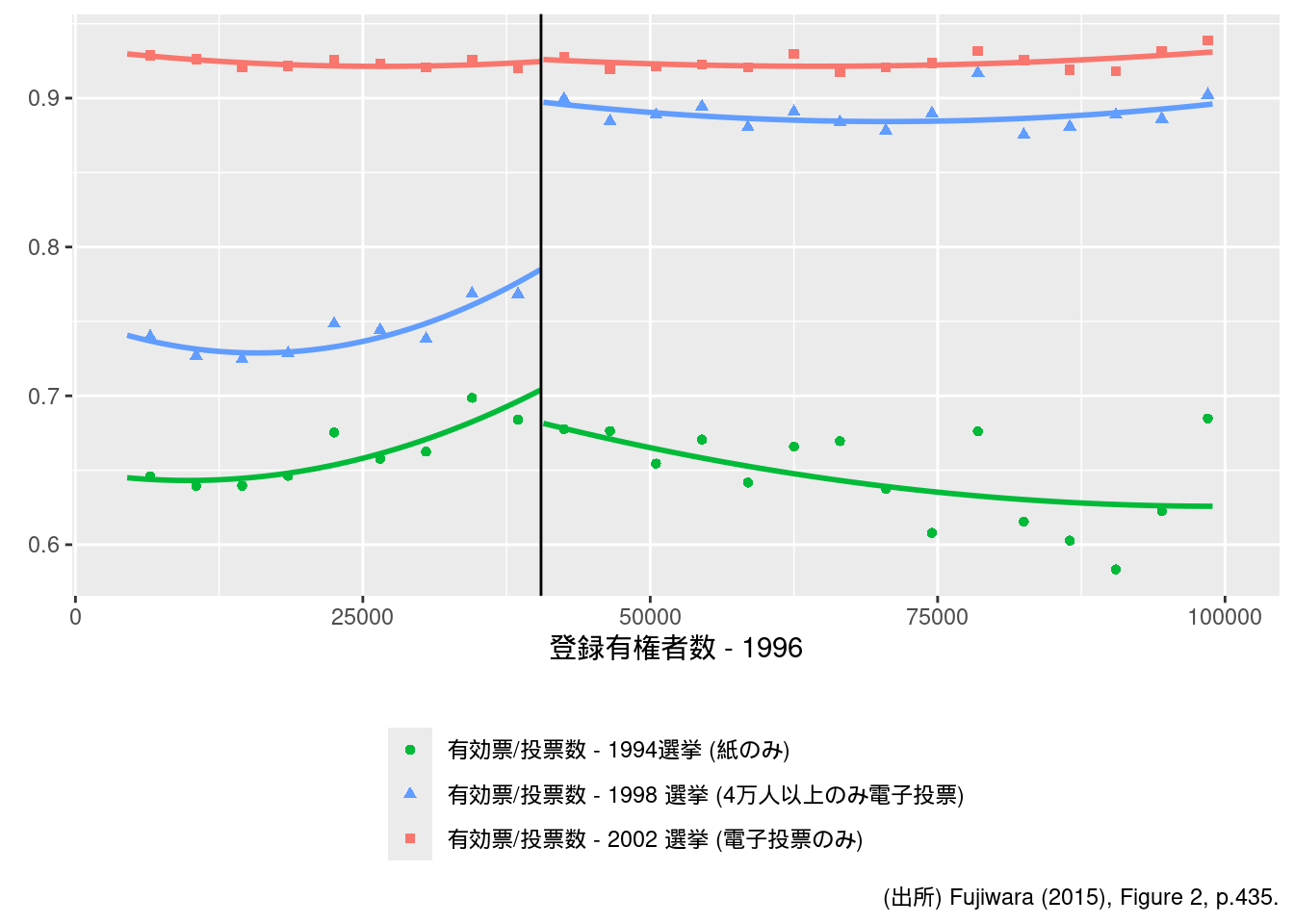
参考までに, 上のようなRDDプロットで変数が1つのみの場合, rdrobust::rdplot()を使うと簡単に描画できる.
また, 変数が2種類の場合上に依存しているパッケージrdmultiを用いることができそうだ.